Introduction to Local Fiber Tracking with EuDX
Published:
Introduction to Local Fiber Tracking with EuDX
Local tractography follows fibers step by step, estimating the local fiber direction at each point from an ODF model. This tutorial covers a full end-to-end local tracking pipeline using DIPY: ODF fitting, stopping criteria, seeding, and the EuDX algorithm.
Dataset
The Stanford HARDI dataset (90 gradient directions, b=2000) is used throughout. DIPY fetches it automatically:
from dipy.data import get_fnames
from dipy.io.image import load_nifti
from dipy.io.gradients import read_bvals_bvecs
from dipy.core.gradients import gradient_table

hardi_fname, hardi_bval_fname, hardi_bvec_fname = get_fnames("stanford_hardi")
data, affine = load_nifti(hardi_fname)
bvals, bvecs = read_bvals_bvecs(hardi_bval_fname, hardi_bvec_fname)
gtab = gradient_table(bvals, bvecs)
Fitting the CSA ODF model
The Constant Solid Angle (CSA) model estimates an ODF at each voxel that captures the fiber orientation distribution:
from dipy.reconst.csdeconv import ConstrainedSphericalDeconvModel
from dipy.reconst.shm import CsaOdfModel

csa_model = CsaOdfModel(gtab, sh_order=6)
csa_fit = csa_model.fit(data, mask=white_matter)
The GFA (Generalized Fractional Anisotropy) map derived from the CSA fit is used to create a binary white matter mask for tracking.
Stopping criterion and seeding
Tracking is constrained to stay within white matter using a GFA threshold:
from dipy.tracking.stopping_criterion import ThresholdStoppingCriterion
from dipy.tracking import utils

stopping_criterion = ThresholdStoppingCriterion(csa_fit.gfa, threshold=0.25)

seeds = utils.seeds_from_mask(cc_slice, affine, density=[2, 2, 2])
Seeds are placed in the corpus callosum at a density of 2x2x2 per voxel.
Running EuDX
EuDX (Euler Delta Crossings) is DIPY’s classic deterministic tracking algorithm:
from dipy.tracking.local_tracking import LocalTracking
from dipy.tracking.streamline import Streamlines
from dipy.direction import peaks_from_model
peaks = peaks_from_model(csa_model, data, sphere, relative_peak_threshold=0.5,
min_separation_angle=25, mask=white_matter)
streamlines_generator = LocalTracking(peaks, stopping_criterion, seeds,
affine=affine, step_size=0.5)
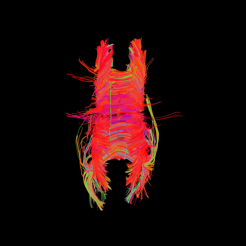
streamlines = Streamlines(streamlines_generator)
The output is a tractogram saved as a .trx file, with visualizations of the direction field and GFA mask shown below.
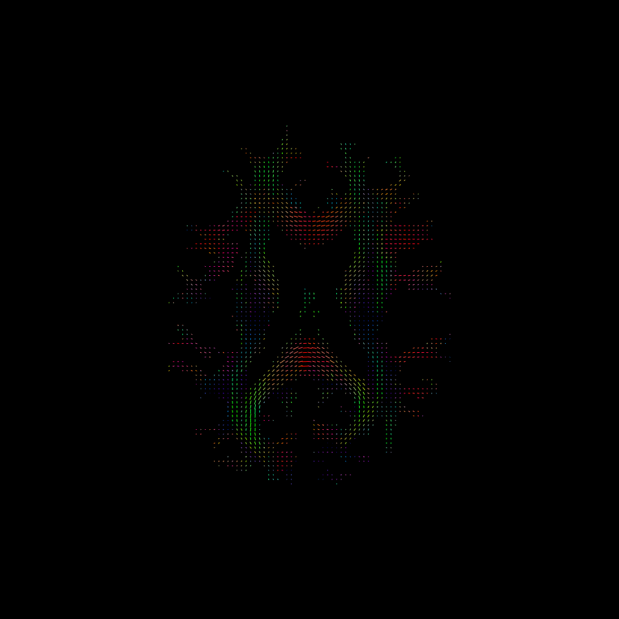
![]()