Extracting the Most Predictive Subgraphs from the Human Connectome

This post is a summary of my Master’s thesis, Extracting Most Predictive Subgraphs From Models of Human Brain Connectivity, submitted in November 2020 for my M.Sc. in Life Science Informatics at the Bonn-Aachen International Center for Information Technology (B-IT), University of Bonn. Examiners: Prof. Dr. Thomas Schultz and Prof. Dr. Holger Fröhlich; advisor: Mohammad Khatami. The full PDF is linked at the bottom.

The problem: dense graphs, few subjects, no interpretability

A structural connectome, built from diffusion MRI tractography, is a graph: brain regions as nodes, white matter fiber bundles between them as edges. With 84 gray matter regions there are 3,486 possible pairwise connections, but a typical study has a few hundred subjects at most. That’s the curse of dimensionality in its most literal form, and it’s compounded by a second problem: even when a classifier trained on this connectivity data works, it doesn’t say why. It’s free to lean on whatever combination of edges numerically separates the classes, whether or not that combination means anything neurobiologically. Filter-based feature selection (keep the top-k edges by some statistical score) doesn’t fix this, since a ranked list of individually-informative edges isn’t the same as a connected subnetwork you can point to and reason about.

The thesis was an attempt to fix that second problem specifically: use graph theory to force the feature selection step to return something structurally interpretable, a connected subgraph, rather than an arbitrary bag of edges.

Building the connectome

Data came from 203 subjects (101 female, 102 male) in the Human Connectome Project’s S900 release. For each subject: probabilistic whole-brain tractography (iFOD2) generated five million streamlines from the diffusion-weighted images, anatomically constrained using a five-tissue-type segmentation of the T1w image, then downsampled to one million biologically-plausible streamlines via SIFT filtering. Combined with an 84-region Desikan-Killiany parcellation (34 cortical + 8 subcortical regions per hemisphere), this gives one connectivity matrix per subject, encoded three different ways: number of streamlines, mean fractional anisotropy (FA), and mean streamline length between every pair of regions.

Of these three, streamline count turned out to be the most useful and most defensible connectivity metric. Mean FA is a local, voxel-level property (it reflects the diffusion tensor’s shape at a single point) and doesn’t translate cleanly into a statement about the strength of a connection between two distant regions. Streamline count, after SIFT’s correction, is instead proportional to the cross-sectional area of the white matter pathway connecting two regions, which gives it a real anatomical meaning. It also happened to produce a cleaner separation between the male and female z-score distributions of the training data than the other two metrics.

Two ways to pick which connections matter

For a given target label (I used gender and, separately, the Big Five personality traits), each of the 3,486 connections gets a score, a t-statistic, f-score, or Pearson correlation, capturing how well that single connection discriminates the classes on the training set. The question is then how to go from those 3,486 scores to a manageable feature set. I compared two approaches:

Baseline. Rank connections by their absolute score and keep the top k%. Simple, standard, and completely blind to graph structure, there’s no requirement that the retained edges form anything connected.

Does the structure actually help?

For gender classification, yes, clearly. Comparing the two techniques at matched numbers of retained edges (streamline count as the connectivity metric, f-scores as the ranking method, SVC as the classifier), the MEWIS-selected subgraph beat the baseline everywhere past a cutoff of about 137 edges, and kept improving as more nodes were added:

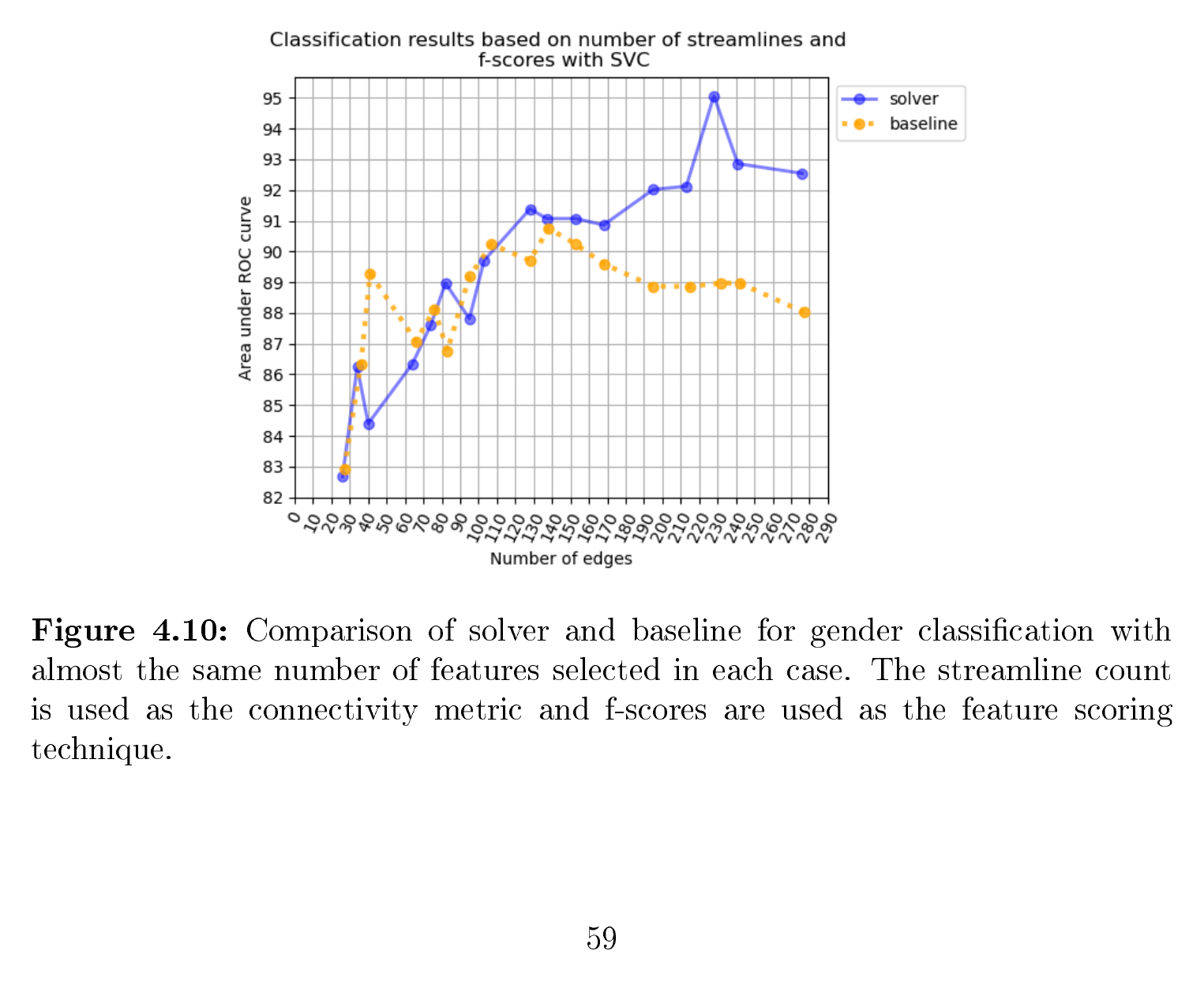
The best solver-based model reached 95% AUC on the independent test set, using a 26-node, 237-edge subgraph; the best baseline model topped out at 91% AUC around 138 edges. Below the 137-edge cutoff the two methods were roughly comparable, so the advantage of the graph-aware approach specifically shows up once you ask it to find a reasonably sized, connected network rather than a handful of individually strong edges.

What made the solver result more than “better AUC,” though, was that the subgraph it returned was inspectable. Six of the ten most important nodes it selected for gender were subcortical, the thalamus, pallidum, hippocampus and caudate, bilaterally, rather than cortical regions:

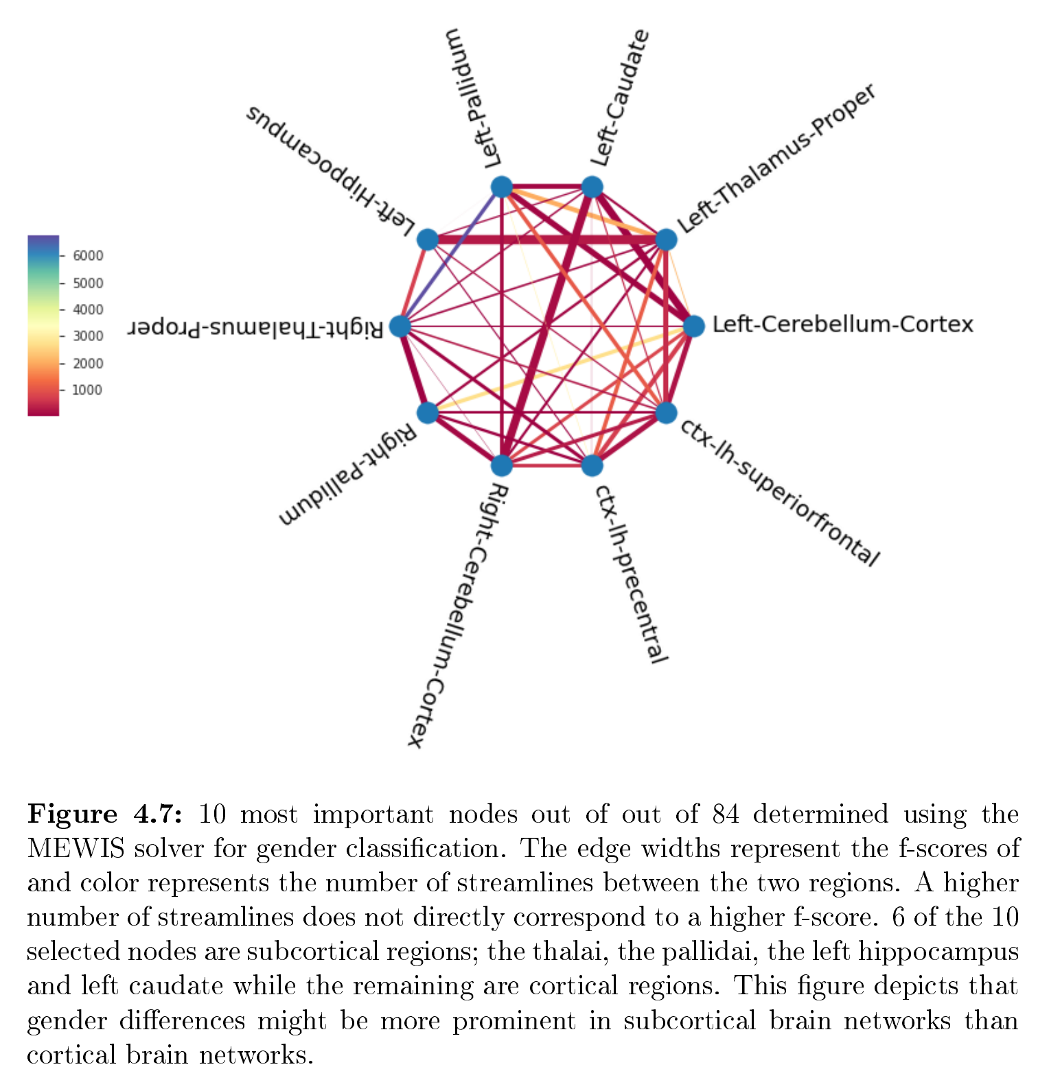
Given that only 16 of the 84 total regions are subcortical, having 6 of the top 10 land there is a real enrichment, not noise. The baseline’s top features, by contrast, preserved almost four times as many nodes (38) for the same number of edges (41), and the resulting graph was disconnected and full of degree-1 nodes, edges that are individually informative but don’t cohere into anything you’d call a subnetwork.

Where it didn’t work: personality traits

I also tried the same pipeline on the Big Five personality traits (agreeableness, openness, conscientiousness, neuroticism, extraversion), binarized around the median after removing subjects in the middle two quartiles. This mostly failed, and I think that failure is itself informative. For openness and conscientiousness, feature selection (of either kind) often did no better, or worse, than using all the features. Only neuroticism and extraversion showed a consistent trend, and even there, the ceiling was modest: the MEWIS solver reached about 64% AUC for neuroticism against a baseline ceiling near 40%, a large relative improvement, but 64% is still a fairly weak classifier. Personality traits inferred from self-report questionnaires may simply not have enough shared variance with structural brain connectivity to be reliably recoverable from ~140 training subjects, which is consistent with the broader replication difficulties reported for MRI-based personality prediction (Dubois et al., 2018).

Retrospective

Looking back at this work, a few things stand out as choices I’d revisit:

The node-weighting trick used to turn the general subgraph problem into a fixed-size one (a small constant negative weight per node) is functional but inelegant; it works only because all edge weights are positive by construction (absolute values of the statistical coefficients), and it took some trial and error to find a magnitude that neither preserved every node nor collapsed the graph entirely.

Binarizing continuous personality scores at the median throws away information before the classifier ever sees the data, and in hindsight a regression-based generative-embedding approach (in the spirit of Brodersen et al.’s DCM work, which I wrote about in a companion post on RBMs and generative embeddings) might have been fairer to the continuous nature of the trait, at the cost of losing the clean subgraph interpretation that motivated the whole project.

And the elephant in the room: this is structural connectivity only. The natural next step, one I gestured at in the conclusion but never ran, is to check whether the subnetworks that predict gender or personality from diffusion MRI overlap at all with the subnetworks that predict the same labels from resting-state functional connectivity. Given how different the failure modes of structural and functional connectomes tend to be, I’d genuinely expect only partial overlap.

Download the full thesis (PDF)

References

• Desikan, R. S., Ségonne, F., Fischl, B., Quinn, B. T., Dickerson, B. C., Blacker, D., Buckner, R. L., Dale, A. M., Maguire, R. P., Hyman, B. T., Albert, M. S., & Killiany, R. J. (2006). An automated labeling system for subdividing the human cerebral cortex on MRI scans into gyral based regions of interest. NeuroImage, 31(3), 968–980.
• Glasser, M. F., Sotiropoulos, S. N., Wilson, J. A., Coalson, T. S., Fischl, B., Andersson, J. L., Xu, J., Jbabdi, S., Webster, M., Polimeni, J. R., Van Essen, D. C., & Jenkinson, M. (2013). The minimal preprocessing pipelines for the Human Connectome Project. NeuroImage, 80, 105–124.
• Bajada, C. J., Schreiber, J., & Caspers, S. (2019). Fiber length profiling: A novel approach to structural brain organization. NeuroImage, 186, 164–173.
• Loboda, A., et al. (2016). Java-based solver for the Generalized Maximum Weight Connected Subgraph problem. github.com/ctlab/gmwcs-solver.
• Smith, R. E., Tournier, J.-D., Calamante, F., & Connelly, A. (2012). Anatomically-constrained tractography: improved diffusion MRI streamlines tractography through effective use of anatomical information. NeuroImage, 62(3), 1924–1938.
• Smith, R. E., Tournier, J.-D., Calamante, F., & Connelly, A. (2013). SIFT: Spherical-deconvolution informed filtering of tractograms. NeuroImage, 67, 298–312.
• Dubois, J., Galdi, P., Paul, L. K., & Adolphs, R. (2018). A distributed brain network predicts general intelligence from resting-state human neuroimaging data. Philosophical Transactions of the Royal Society B, 373(1756).