Modeling Why the Necker Cube Won’t Sit Still

Most write-ups of visual illusions stop at showing you the picture: here’s a cube that flips, isn’t the brain weird. That’s true but incomplete, it doesn’t say why perception should flip at all, rather than just settling on one interpretation and staying there, or why the flips arrive when they do rather than on some fixed schedule. This post builds a small computational model of exactly that switching process, for the Necker cube specifically, and asks whether a handful of very simple neural dynamics can reproduce the statistical signature of real perceptual switching.

The phenomenon

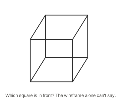
The Necker cube (Necker, 1832) is a wireframe drawing of a cube with no occlusion, shading, or perspective cues, so nothing in the image itself specifies which of the two squares is “in front.” Look at it for a while and your perception of depth spontaneously flips between the two readings, unprompted, every few seconds. This is bistable perception, and the Necker cube is one instance of a broader family that includes Rubin’s vase, binocular rivalry, and ambiguous motion displays. What’s been established since Levelt’s foundational work on binocular rivalry (Levelt, 1965) is that these switches are not periodic. Dominance durations, how long one interpretation holds before flipping, are irregular and right-skewed: lots of short-to-medium durations, a long tail of occasional long ones, and almost never a duration close to zero. That specific statistical shape is the target I wanted a toy model to reproduce, not just “it flips sometimes.”

A minimal neural model

The standard account (Moreno-Bote, Rinzel, & Rubin, 2007) treats bistable perception as the output of two neural populations, one per interpretation, that mutually inhibit each other, each with its own slow self-adaptation, plus noise. Written as two coupled rate equations:

where $r_1, r_2$ are the two populations’ activity, $\sigma$ a sigmoid nonlinearity, $I_0$ an equal, constant, ambiguous drive to both, $w$ the mutual inhibition strength, $a_1, a_2$ slow self-adaptation terms (each population fatigues in proportion to its own recent activity, at a much slower timescale $\tau_a \gg \tau_r$), and $\xi_1, \xi_2$ independent noise. There’s no image of a cube anywhere in this, $r_1$ and $r_2$ are just abstract labels for “interpretation A dominant” and “interpretation B dominant.”

The interesting part, which took some parameter-hunting to find, is that this system has two qualitatively different regimes. With strong adaptation, the noise-free system ($\xi = 0$) oscillates on its own: population 1 wins, fatigues, loses to population 2, which then fatigues in turn, and so on forever, like a relaxation oscillator. That regime produces switches, but almost perfectly periodic ones, nothing like real perception. Turn the adaptation gain down far enough, and the noise-free system instead settles permanently into whichever population won first, true bistability, no autonomous switching at all. Add noise back into that regime, and switching becomes noise-driven: fluctuations occasionally let the suppressed population escape inhibition, with adaptation only making that escape gradually more likely the longer a population has been on top. It’s this second, noise-driven regime, not the oscillator, that turned out to reproduce the right statistical shape.

def simulate(T=1500.0, dt=0.01, tau_r=0.2, tau_a=3.0, w_inhib=5.0,
             a_gain=0.5, I0=2.5, noise_sigma=0.6):
    n_steps = int(T / dt)
    r1, r2, a1, a2 = 0.6, 0.4, 0.0, 0.0
    r1_trace, r2_trace = np.zeros(n_steps), np.zeros(n_steps)

    for t in range(n_steps):
        noise1, noise2 = np.random.normal(0, noise_sigma, 2)
        dr1 = (-r1 + sigmoid(I0 - w_inhib * r2 - a1 + noise1)) / tau_r
        dr2 = (-r2 + sigmoid(I0 - w_inhib * r1 - a2 + noise2)) / tau_r
        da1 = (-a1 + a_gain * r1) / tau_a
        da2 = (-a2 + a_gain * r2) / tau_a
        r1 += dt * dr1; r2 += dt * dr2
        a1 += dt * da1; a2 += dt * da2
        r1_trace[t], r2_trace[t] = r1, r2

    return r1_trace, r2_trace

To read “which percept is dominant” off the resulting traces, a plain zero-crossing of $r_1 - r_2$ isn’t enough, noise near a crossing produces bursts of spurious near-instantaneous flips that aren’t real perceptual reversals. I used a small hysteresis margin instead (switch state only once one unit leads the other by some threshold $\theta$, à la a Schmitt trigger), which is a modeling choice worth being upfront about rather than something the dynamics hand you for free.

Results

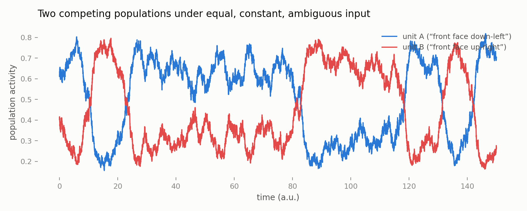
Simulating 1,500 time units in this noise-driven regime gives an activity trace that alternates irregularly, long stretches of dominance next to short ones, with no fixed period:

Extracting all 83 dominance durations from a longer run and histogramming them gives a right-skewed, unimodal distribution (mean 17.7, median 13.0, so mean/median ≈ 1.36), lots of short-to-medium durations and a long tail out past 60:

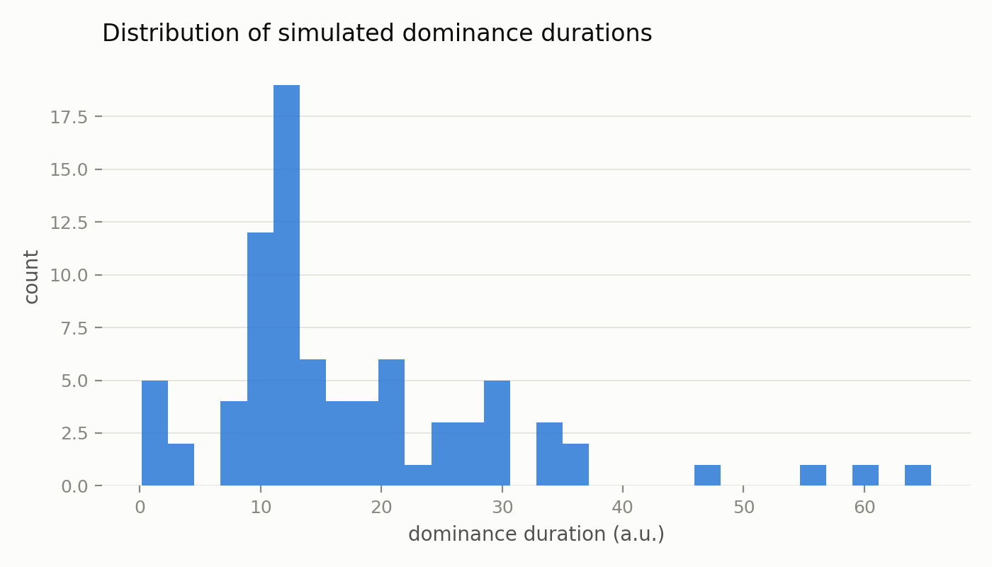
That mean/median ratio above 1 is the qualitative signature Levelt’s work established for real binocular rivalry and bistable figures generally, and it’s not a foregone conclusion: it only emerges from this model in the noise-driven parameter regime, not the oscillator regime, and I only found that distinction by hunting through parameters and checking which ones gave a genuinely bistable (rather than autonomously oscillating) noise-free system first.

Toy in every sense

Two abstract rate units are not a visual system. There’s no actual image of a cube anywhere in this model, no encoding of edges or depth cues, just two labels competing for an arbitrary equal drive; whatever makes “front-square-down-left” and “front-square-up-right” the two specific hypotheses on offer is entirely outside this model’s scope. The parameters (inhibition strength, adaptation gain, noise level) were hand-tuned to get a plausible qualitative shape, not fit to any published dataset, and the hysteresis threshold used to strip out sub-crossing noise flicker is a modeling choice I imposed, not something the dynamics produce unassisted. Real bistable perception is also known to respond to voluntary attention (you can, within limits, hold one interpretation longer by trying), which this model has no mechanism for at all.

It’s also worth naming the family this belongs to: mutual inhibition plus slow adaptation plus noise is one story for why perception switches, essentially a mechanical, bottom-up account. A different, top-down story, in the spirit of predictive coding and the free energy principle, would frame the two interpretations as competing hypotheses in a generative model, with perception flipping to whichever hypothesis currently best explains the ambiguous input, and switching driven by accumulating prediction error rather than neural fatigue. The two accounts aren’t mutually exclusive, and reconciling them (does adaptation implement approximate Bayesian inference, or are they genuinely separate mechanisms operating on the same phenomenon) is an open enough question that it’s fair to just flag it here rather than pretend this toy model settles it.

References

• Necker, L. A. (1832). Observations on some remarkable phenomena seen in Switzerland; and an optical phenomenon which occurs on viewing a figure of a crystal or geometrical solid. The London and Edinburgh Philosophical Magazine and Journal of Science, 1(5), 329–337.
• Levelt, W. J. M. (1965). On Binocular Rivalry. Institute for Perception RVO-TNO.
• Leopold, D. A., & Logothetis, N. K. (1999). Multistable phenomena: changing views in perception. Trends in Cognitive Sciences, 3(7), 254–264.
• Moreno-Bote, R., Rinzel, J., & Rubin, N. (2007). Noise-induced alternations in an attractor network model of perceptual bistability. Journal of Neurophysiology, 98(3), 1125–1139.